Kaman Inductive Technology Applications Guide
|
KAMAN PRECISION PRODUCTS / MEASURING |
|
| Kaman Precision Products / Measuring is a division of Kaman Aerospace Corporation. Kaman Corporation has over 60 years experience as a leader in aerospace, industrial, military, and consumer products. Kaman Precision Products / Measuring draws on over 40 years of experience with inductive position measurement techniques to bring you the best in advanced sensor technology and signal conditioning electronics.
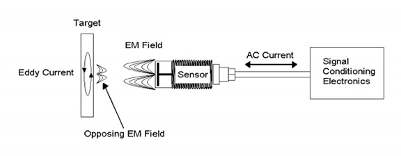
Our Location TABLE OF CONTENTS SECTION 1 – INTRODUCTION 4 SECTION 2 – NON CONTACT MEASURING TECHNOLOGIES 5 SECTION 3 – INDUCTIVE TECHNOLOGIES OVERVIEW 7 SECTION 4 – APPLYING INDUCTIVE MEASURING SYSTEMS 16 SECTION 5 – PERFORMANCE 26 APPENDIX A CALIBRATION TERMINOLOGY 30 APPENDIX B SENSOR MOUNTING GUIDELINES 33 APPENDIX C TYPICAL TARGET MATERIAL CHARACTERISTICS 36 GLOSSARY 37 QUICK CONVERSION 39 Section 1 – Introduction Numerous textbooks, handbooks, and assorted publications are available on sensor technology. These documents typically cover a broad range of sensors and technologies, but have limited information on each type. Information on inductive sensors can be found in many of them. This handbook is different in that it condenses technical and application information on inductive sensors into a single source. The intent is to help the reader understand where inductive sensors can be utilized, how to best apply them, and to understand their performance. Why Kaman? We are the “high-end” guys in the inductive world! When you have a demanding measurement application, call your Kaman Applications Engineer, . . .that’s Kaman, pronounced “Ca’•man.” Section 2 – Non Contact Measuring Technologies There are many instruments to measure position, distance, or vibration of an object. These can be segregated into two basic categories: contact and non-contact. Popular contact methods are: Linear Encoders, String Potentiometers, and Linear Variable Displacement Transducers (LVDTs). Some of the benefits of contact measuring systems are: long measuring range, target material insensitivity, a small spot (measuring area) size, and generally lower cost. While contact instruments are suitable for many applications, they have a limited frequency response and can interfere with the dynamics of the object being measured. Where these factors are a concern, non contact methods have advantages. Below is a list of several types of non contact measuring technologies with some of their features. Air Gauging: This technique uses air pressure and flow to measure dimensions or inspect parts. These devices operate on changes in pressure and flow rates to make a measurement. A clean air supply is required. It is acceptable for use on most target materials and typically used for small measuring ranges of 0.010 to 0.200 inches in production environments. Hall Effect: This sensor varies its output voltage in response to changes in magnetic field. With a known magnetic field, distance can be determined. A magnetic target or attachment of a magnet to the target is required. These sensors are generally inexpensive and are used in consumer equipment and industrial applications. They are also commonly used in automotive timing applications. Ultrasonic: Ultrasonic sensors operate on a principle similar to sonar by interpreting echoes of sound waves reflecting off a target. A high frequency sound wave is generated by the sensor and directed toward the target. By calculating the time interval between the sent and received signals, distance to the target is determined. Ultrasonic sensors have long measuring ranges and can be used with many target materials, including liquids. Performance is affected by shape and density of the target material. They have lower resolution than most other non-contact technologies and cannot work in a vacuum. Ultrasonic sensors are frequently used to measure liquid level in tanks and in factory automation and process industries. Photonic: Photonic sensors use glass fibers to transmit light to and from target surfaces. Displacement is determined by detecting the intensity of the reflected light. These sensors have a very small spot size and can be used to detect small targets. They can be used with most target materials and in hostile environments. They are also insensitive to interference from EMI or high voltages. Photonic sensors are generally used for small measuring ranges and can have high resolution and frequency response. But, they are sensitive to environmental contaminants and target finish variations. Capacitance: These sensors work on the principal of capacitance changes between the sensor and target to determine distance. They can be used with all conductive target materials and are not sensitive to material changes. Capacitive sensors have a relatively small spot size and are not sensitive to material thickness, but typically require a target grounded to the measuring system. They can be constructed of very high temperature materials for measurements up to 1200oC. These sensors have a small measuring range to sensor diameter ratio and are sensitive to environmental changes and contamination. Laser Triangulation: These sensors work by projecting a beam of light onto the target and calculating distance by determining where the reflected light falls on a detector. They can measure longer ranges than other non-contact technologies; can be used with most target materials, and have a very small measuring spot size. They tend to be the most expensive type of non-contact sensor. Measurement is affected by environmental contamination and surface finish variations of the target. Inductive Eddy Current: Inductive eddy current sensors operate by generating a high frequency electro-magnetic field about the sensor coil, which induces eddy currents in a target material. A conductive target is required, but a ground connection to the measuring system is not necessary. Sensor performance is affected by target material conductivity. Inductive sensors have a large spot size in comparison to other technologies. Performance is affected by temperature changes, but not by environmental contaminants or target finish characteristics. They can operate in a vacuum or in fluids. Non-conductive material between the sensor and the target is not detected. The measuring distance is typically 30-50% of sensor diameter. As with any device, both contact and non-contact measuring technologies have a wide range of performance characteristics ranging from very low (on-off) to very high precision (nanometer resolution), depending on their construction. It is not only necessary to choose the correct technology, but also the correct level of performance for an application. Section 3 – Inductive Technologies Overview 3.1 Basic Inductive Technology Basic inductive measurement technology must first be understood before it can be successfully applied. The operational concept is simple; however, many different parameters can affect system performance. The application of this technology should be approached in a logical step-by-step manner which will insure that all parameters are considered. An AC current flowing in a coil generates a pulsating electromagnetic field. Placing the coil a nominal distance from an electrically conductive “target” induces a current flow on the surface and within the target. This induced current is called “eddy current”. The eddy current produces a secondary magnetic field that opposes and reduces the intensity of the original field. This interaction is called the “coupling effect.” The strength of the electromagnetic coupling between the sensor and target depends upon the gap between them. Signal conditioning electronics sense the effects of impedance variations as the gap changes and translate them into a usable displacement signal.
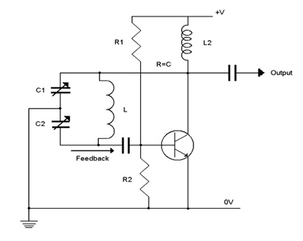
In the previous section, we discussed the basics of how eddy current works in interaction with sensor and target. The following is a discussion of how those eddy currents can be interpreted and processed into useful information in the signal conditioning electronic circuits. There are three popular types of circuits used to process the signal. These are: COLPITTS CIRCUIT – Single Channel Analog Position Measuring Systems BALANCED BRIDGE CIRCUIT – Single Ended & Differential Analog Linear Position Measuring Systems PHASE CIRCUIT – Single/Multiple Channel Analog High Precision Position Systems Each of these circuits has distinct characteristics. The signal conditioning circuit that performs best in any application should be chosen. Details of each circuit are discussed in the following sections. 3.2 Colpitts Circuit Theory of Operation
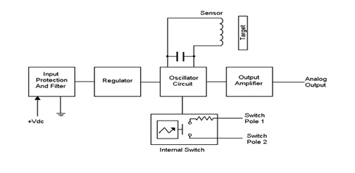
When used as a position measuring device, the sensor coil becomes the inductor in the oscillator circuit. When the sensor coil interacts with a conductive target, the oscillator frequency and amplitude vary in proportion to the target position. This variation is processed into an analog signal proportional to displacement. The basic block diagram of a circuit using this technology is shown below.
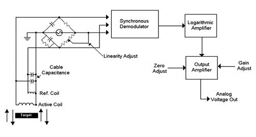
Applications A Colpitts inductive proximity measuring system is a rugged, low cost, non-contact measuring system with good resolution and repeatability for static and dynamic measurements. Output is a non-linear DC voltage signal proportional to the distance between the sensor and the target. A single adjustment for gain control is used to raise or lower the output voltage level to the desired value. This circuit does not have provisions for control of offset or linearity of the output signal. A Colpitts circuit can be used in a variety of applications with performance quite different from other inductive technologies. This circuit responds to any conductive material, but very well to magnetic steel and highly resistive targets. In general, a Colpitts circuit provides a larger measuring range for the same size sensor than other types of inductive circuits. While output is non-linear over the total range of a sensor, it can be very linear if only a small portion of the range is used in an application and is very repeatable. Using a Colpitts inductive measuring system, things to consider are: Typical applications are: Systems 3.3 Balanced Bridge Circuit Theory of Operation The target movement causes an impedance change in the sensor coil. This change of impedance in the coil is detected (measured) by the demodulator circuit, linearized by a logarithmic amplifier, and then amplified in the final amplifier stage, which provides offset and gain. This voltage is the system output voltage, provided to the user as an analog voltage directly proportional to target position relative to the sensor.
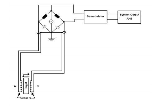
In the single ended configuration, the bridge circuit can be used with both dual and single coil sensors. In the dual coil design, the active and inactive coils are on opposing sides of the bridge. This configuration provides a “canceling” effect, which can enhance some performance parameters. In the single coil configuration, only one coil is exposed to the measuring environment. While the impact of the environment may be greater, the stabilization time will be shorter.
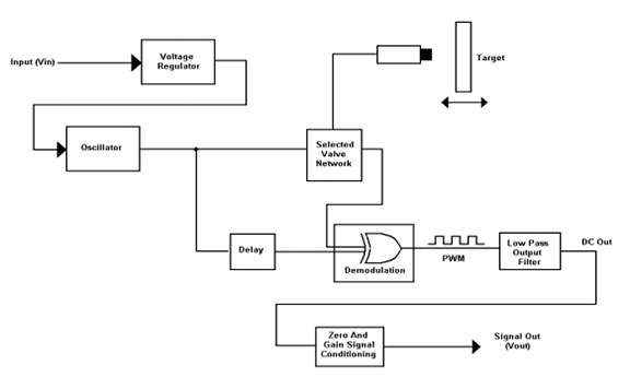
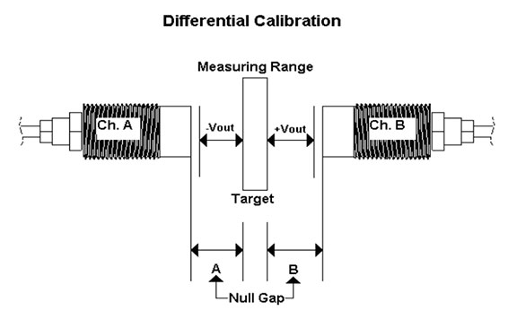
In the differential configuration, two sensors are used to sense target movement. Two single coil sensors are mounted on either side of a target and are connected to opposite sides of the balanced bridge. When the target is electrically centered between the two sensors, the bridge is balanced and system output is zero. This position is called the “null gap”. As the target moves toward one sensor and away from the other, the bridge becomes unbalanced and outputs a proportional analog voltage, which indicates both the magnitude and direction of movement. This bipolar (A-B) signal is a true differential output. Individual sensor outputs are not available from this type of system. The differential configuration is more difficult and costly to implement since it requires two sensors for a single measurement. However, compared to a single ended configuration, it does offer some distinct advantages: When the target is electrically centered between the two sensors at the nominal null gap for each, the system output is zero. As the target moves away from one sensor and toward another, the coupling between each sensor and target is no longer equal; causing an impedance imbalance and its output is amplified, demodulated, and presented as a linear analog signal directly proportional to the target’s position. This is a bipolar signal that provides both magnitude and direction of misalignment. Only A-B or differential output is available. Applications These single ended systems were developed to satisfy an extremely wide variety of measurement applications for both ferrous and non-ferrous targets, including: Applications for differential bridge systems include: Bridge Circuit Systems The KD-2306 is a single ended, high precision position measuring system. It can be configured with both dual and single coil sensors. There are 3 outputs available: single ended analog voltage, differential analog voltage (not to be confused with differential measurements), and a 4 to 20 mA current output. The KDM-8206 is a single ended, multi-channel system which utilizes the same basic circuitry as the KD-2306. It is available in one-half, three-fourths, and full 19-inch instrumentation rack configurations of up to 12 measuring channels. Differential Systems The KD-5100 is a differential measuring system which was developed to satisfy the demands of high precision military measurement applications. It has a history of use in a variety of high precision/high reliability industrial applications as well. The DIT-5200 is a lower priced equivalent commercial version of the KD-5100, incorporating COTS (Commercial Off The Shelf) parts in a small commercial electronics enclosure. The DIT-5200 is available with several sensor options suitable for high precision applications. The system provides a DC voltage output. It is intended for low to high volume end user applications and is very well suited to high precision OEM applications. 3.4 Phase Circuit Theory of Operation The effects of eddy currents are not only amplitude related, but also phase related. This circuit is based on phase detection as opposed to amplitude detection. Specifically, the phase detection is based on Pulse Width Modulation (PWM) techniques. Since noise is basically an amplitude sensitive phenomenon, the phase detection technique offers a lower noise floor to begin with. In systems utilizing the amplitude changes, the system is full of op-amps with their inherent noise. The PWM technique used does not require high gain op-amps, which allows for extraordinary low noise on the system output. The proprietary PWM circuit allows for the optimization of temperature stability or linearity.
Applications Applications span many areas, including new product research and design, manufacturing process control, and part fabrication and inspection, where the application requires high resolution. Typical applications are: Systems The Kaman SMT-9700 series is a PWM based system. This system has a small footprint, is ideal for OEM configurations, has excellent resolution, and only requires a single ended power supply. Custom designs can be tailored to meet the customers needs, and 18 pin, SIP (Single In-line Package) cards are available for customers to integrate into existing motherboards. Section 4 – Applying Inductive Measuring Systems The acronym “TERMS” is a simple way to ensure that you have covered the fundamentals when applying an inductive measuring system. TERMS stand for Target, Environment, Range, Mounting, and Speed. This section addresses each of these fundamentals in detail. 4.1 Target What type of material makes a good target? Since the inductive principle relies on an opposing current to be induced in the surface of the target material, it stands to reason that a good target should be highly conductive and have uniform electrical characteristics. Material Properties Magnetism Thickness Size and Shape
A general rule for cylindrical targets, such as a shaft, is to use a sensor that is 8 to 10 times smaller in diameter than the shaft diameter. This will make the shaft appear as an infinite plane. If the shaft is smaller than recommended, the system will be more sensitive to cross axis variation (errors caused by side to side movement of the target, which in turn creates non uniform eddy current coupling with the target).
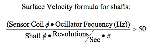
Surface 4.2 Environment In general, inductive systems are well suited for all types of environments. Kaman offers sensors that operate when submerged in diesel fuel, oil, grease, antifreeze, brake fluids, machining oils, and even salt water. Kaman sensors are available that operate from cryogenic to 1100° F; however, special consideration must be given when operating over wide temperature ranges to insure optimum performance. Temperature Temperature variations at the sensor/target interface may cause thermal sensitivity shift, which affects gain and linearity. A factory temperature compensation option will minimize the effect on the thermal sensitivity shifts. Resetting the zero control corrects thermal zero shift. This occurs when temperature changes cause the resistivity in the sensor or cable to change. The zero control does not correct sensitivity shift. Pressure Pressure and vacuum do not affect performance of an inductive sensor. However, special consideration must be given to select a sensor that can survive and, if necessary, seal to the pressure boundary. Vibration As a general rule, standard Kaman sensors can withstand 100 G shock (1200 mSec, half sine wave) and 10 G peak vibration (20 Hz – 2 kHz sinusoidal), without significant performance degradation. Empirical studies have shown that system output is affected by less the 1% of full scale output after being subjected to the above. The sensors used for testing were large diameter (>1.00 inch), hence, small, lower mass sensor could in theory withstand higher levels of vibration and shock without a significant degradation in performance. Fluids EMI (Electro-Magnetic Interference) EMI due to sensor-to-sensor proximity is addressed in the sensor mounting section of this handbook (refer to Appendix B). Interference from electro-magnetic fields present in the environment may or may not be a problem depending on their frequency and strength. Inductive sensors are typically excited with 1 MHz or 500 KHz carrier signals. In general, interferences that are not within +/- 10% of the carrier are filtered out by the demodulator circuit in the electronics. The demodulator may not filter out very strong fields (such as near windings of an electric motor), regardless of the frequency. For signals close to the operating frequency of the sensor or strong fields, shielding around the sensor to mitigate the field is the only way to reduce interference. If a sensor must operate in an electro-magnetic field, non-ferrous target materials are recommended. Ferrous targets can experience permeability changes due to the field which will also be a source of error. 4.3 Range Measuring Range An example is a sensor with a 0.120 inch coil diameter has an effective measurement range of 0.040 inch and a sensor with a coil diameter of 3.00 inch has an effective measurement range of 1.20 inch. Space constraints often dictate the sensor diameter and mounting configuration. Because measuring range is proportional to sensor size, it affects sensor selection. Larger sensors provide greater measuring range, but typically less absolute resolution than a smaller sensor. Using only a portion of a sensor’s measuring range high accuracy-band calibration improves overall performance. Offset Sensor/target should never go inside the offset. An offset is necessary to keep the sensor a non-contact device, and to put the sensor inductive characteristics in a more linear portion of its range. Refer to Calibration Terminology in Appendix A. 4.4 Mounting The quality of any measurement depends on the mounting fixture. Unstable or nonrepeatable fixturing will yield non-repeatable results. Fixture For more information on Fixturing refer to Appendix B. Non Parallelism Sensor to Sensor Proximity 4.5 Speed Surface Velocity
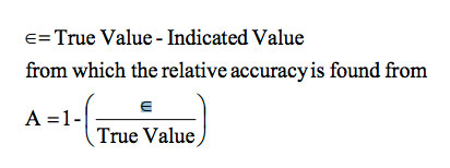
If the above equation is satisfied, the system should provide less than 1% error due to surface velocity. Event Detection 4.6 “TERMS” – Summary TARGET Material Properties Magnetism Thickness Size/Shape Surface ENVIRONMENT Temperature Pressure Vibration RANGE Measuring Range MOUNTING Fixture Sensor to Sensor Proximity SPEED Surface Velocity Event Detection Section 5 – Performance The performance of a system encompasses several different parameters, including; Output/Sensitivity, Resolution, Frequency Response, Non Linearity, Stability, and Accuracy. This section addresses each of these in detail. 5.1 Output/Sensitivity 5.2 Resolution 5.3 Frequency Response 5.4 Non Linearity This is basically an error, or deviation from the theoretical straight-line output signal from the offset position to the maximum calibrated position. In applications that evaluate a movement for a force applied, a highly linear system may be desirable. In applications where the desire is to repeat a given position, linearity can be a rather insignificant specification. (Non-linearity is typically expressed in least squares deviation from a best fit line). 5.5 Stability The stability of a system can be impacted by several factors, two of which are temperature and electronics. Thermal Stability Long Term Stability Although Long Term Stability is inherent in the electronics, there are external influences such as fixturing which can have an impact. Therefore, the first step in resolving drift problems is to eliminate the external influences. Where Long Term Stability is a concern for the measurement, components such as potentiometers can be replaced with fixed resistors in some circuits. 5.6 Accuracy The accuracy of a measurement system refers to its ability to indicate a true value exactly. Accuracy is related to absolute error. Absolute error ( ) is defined as the difference between the true value applied to a measurement system and the indicated value of the system:
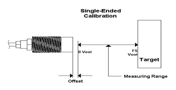
Based on this definition, accuracy can be determined only when the true value is known, such as during a calibration. An inductive system’s accuracy can be adversely affected by several parameters (error source), including: temperature, nonlinearity, target frequency, and fixturing. Kaman does not provide system accuracy specifications since all of the parameters cannot be replicated for each specific application in the calibration laboratory. APPENDICES Appendix A Calibration Terminology There are 3 basic calibrations: Single-Ended, Bipolar, and Differential. The following information and illustrations provide a description of the calibration, the definitions of the terminology used to specify the calibration parameters, and an example of the calibration specification. Single-Ended Calibration • Offset: The closest the target will come to the sensor Example of Single-Ended Calibration Specification:
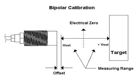
Bipolar Calibration • Offset: The closest the target will come to the sensor Example of Bipolar Calibration Specification:
Differential Calibration • Null: The distance between the sensor face and the target at which the output is 0 Vdc Example of Differential Calibration Specification:
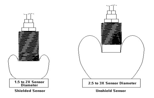
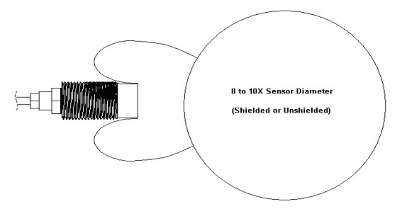
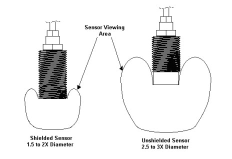
Appendix B Sensor Mounting Guidelines The electromagnetic field (field) emitted by the sensor is omni-directional. Its size and shape is a function of the coil design, the shielding, and the application mounting configuration. Conductive material other than the target entering into the field causes “side-loading”. The most common form of side-loading comes from the counting configuration. Side-loading of the field can reduce the range of a sensor by as much as 50%. If the loading extends beyond the face of the sensor, the impact will be even greater. Sensors may be classified as either shielded or unshielded. A shielded sensor is designed with a metal housing extending to the face of the sensor. An unshielded sensor is designed so that the metal housing stops some distance behind the face of the sensor. The illustration below shows the effects of the sensor housing shielding on the size and shape of the field.
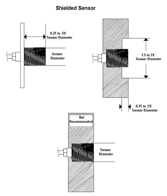
Shielded Sensors The illustration below provides guidelines for mounting shielded sensors.
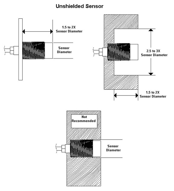
Unshielded Sensors
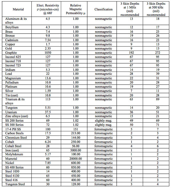
Appendix C Typical Target Material Characteristics
Glossary Analog Output Coupling Effect Cross Axis Dimensional Standard Drift Effective Resolution Equivalent RMS Input Noise Full Scale Output (FSO) Gain Iteration = Repetition. Linearity Loading Measurement Bandwidth Noise Offset Output Pass Line Range Repeatability Resolution Target QUICK CONVERSION 1 Mil 1 Millimeter |
|